
Training a neural network boils down to two fundamental operations that repeat over and over: forward propagation (making a prediction) and backward propagation (learning from the mistake). Together, they form the heartbeat of every deep learning model — from a simple perceptron to GPT-scale transformers.
In this article, we will walk through both processes step by step with concrete math, intuitive diagrams, and a from-scratch Python implementation.
1. The Setup: A Simple Neural Network
Consider a minimal neural network designed to learn the XOR function — a classic problem that a single-layer perceptron cannot solve, but a network with one hidden layer can.
Our network architecture:
- Input Layer: 2 neurons ($x_1$, $x_2$)
- Hidden Layer: 3 neurons with Sigmoid activation
- Output Layer: 1 neuron with Sigmoid activation
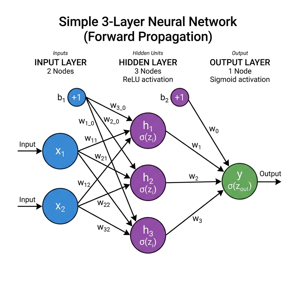
Every connection between neurons carries a weight ($w$), and every non-input neuron has a bias ($b$). These are the parameters the network will learn.
2. Forward Propagation — Making a Prediction
Forward propagation is the process of passing input data through the network, layer by layer, until an output (prediction) is produced. At each neuron, two things happen:
Step 1: Weighted Sum (Linear Transformation)
Each neuron computes a weighted sum of its inputs plus a bias term:
$$z = \sum_{i} w_i \cdot x_i + b$$
For example, for hidden neuron $h_1$ with inputs $x_1 = 0$ and $x_2 = 1$:
$$z_{h_1} = w_{11} \cdot x_1 + w_{12} \cdot x_2 + b_1$$
If $w_{11} = 0.5$, $w_{12} = -0.3$, and $b_1 = 0.1$:
$$z_{h_1} = (0.5)(0) + (-0.3)(1) + 0.1 = -0.2$$
Step 2: Activation Function (Non-Linear Transformation)
The weighted sum $z$ is then passed through an activation function to introduce non-linearity. Using the Sigmoid function:
$$\sigma(z) = \frac{1}{1 + e^{-z}}$$
$$a_{h_1} = \sigma(-0.2) = \frac{1}{1 + e^{0.2}} \approx 0.4502$$
This process repeats for every neuron in the hidden layer, then again for the output layer. The final output neuron produces the network's prediction $\hat{y}$.
Step 3: Compute the Loss
After forward propagation produces a prediction $\hat{y}$, we compare it to the true label $y$ using a loss function. For binary classification, we commonly use Mean Squared Error (MSE):
$$\mathcal{L} = \frac{1}{2}(y - \hat{y})^2$$
If $y = 1$ (true label) and $\hat{y} = 0.62$ (our prediction):
$$\mathcal{L} = \frac{1}{2}(1 - 0.62)^2 = \frac{1}{2}(0.1444) = 0.0722$$
The loss tells us how wrong the prediction is. The goal of training is to minimize this value.
3. Backward Propagation — Learning from Mistakes
Backpropagation is the algorithm that computes how much each weight contributed to the error, so we know exactly how to adjust it. It works by applying the chain rule of calculus to propagate gradients from the output layer back through every layer of the network.
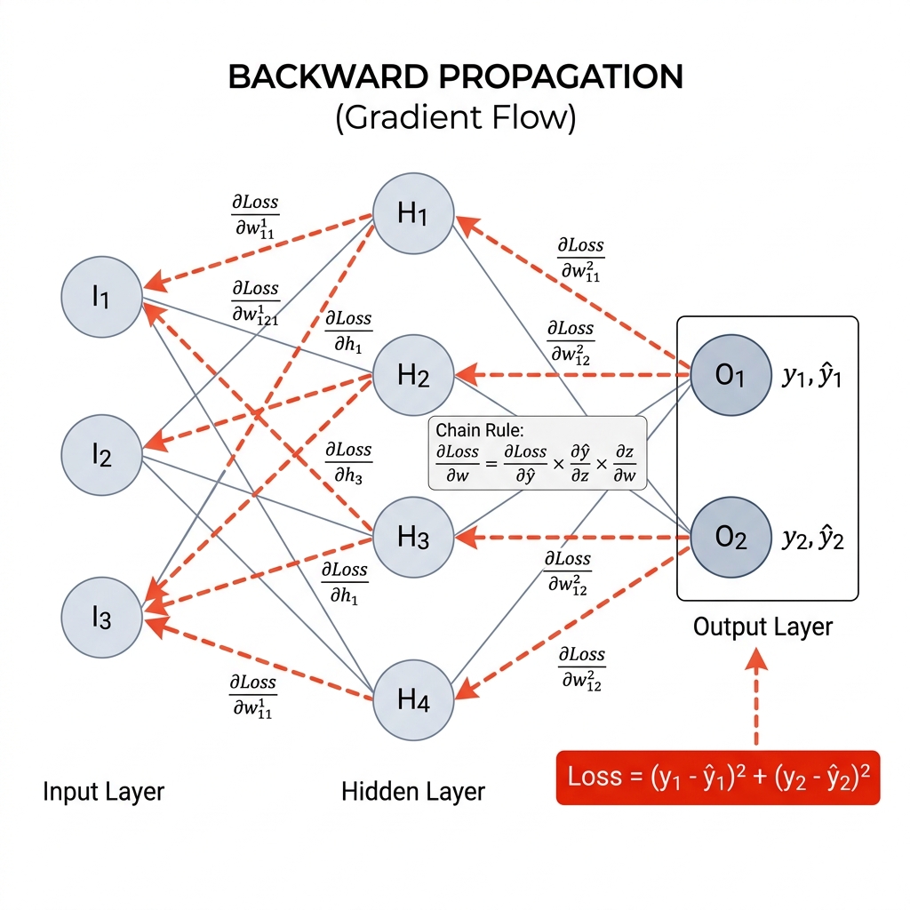
The Chain Rule — The Core Engine
To update a weight $w$, we need to know: "How much does the total loss change if I nudge this weight by a tiny amount?" Mathematically, that is the partial derivative $\frac{\partial \mathcal{L}}{\partial w}$.
Since the loss depends on the output, which depends on the weighted sum, which depends on the weight, we chain these derivatives together:
$$\frac{\partial \mathcal{L}}{\partial w} = \frac{\partial \mathcal{L}}{\partial \hat{y}} \cdot \frac{\partial \hat{y}}{\partial z} \cdot \frac{\partial z}{\partial w}$$
Computing Each Piece
1. Loss w.r.t. prediction:
$$\frac{\partial \mathcal{L}}{\partial \hat{y}} = -(y - \hat{y}) = -(1 - 0.62) = -0.38$$
2. Prediction w.r.t. weighted sum (derivative of Sigmoid):
$$\frac{\partial \hat{y}}{\partial z} = \hat{y}(1 - \hat{y}) = 0.62 \times 0.38 = 0.2356$$
3. Weighted sum w.r.t. weight:
$$\frac{\partial z}{\partial w} = a_h \quad \text{(the activation from the previous layer)}$$
Multiplying them together gives the gradient for that specific weight.
Updating the Weights
Once we have the gradient, we update the weight using gradient descent:
$$w_{\text{new}} = w_{\text{old}} - \alpha \cdot \frac{\partial \mathcal{L}}{\partial w}$$
Where $\alpha$ is the learning rate — a hyperparameter that controls how large each step is. Too large and you overshoot; too small and training takes forever.
4. The Training Loop
Training a neural network is simply repeating these two phases thousands or millions of times:
- Forward pass: Compute prediction $\hat{y}$ and loss $\mathcal{L}$
- Backward pass: Compute gradients $\frac{\partial \mathcal{L}}{\partial w}$ for all weights
- Update: Adjust all weights using gradient descent
- Repeat until the loss converges to a minimum
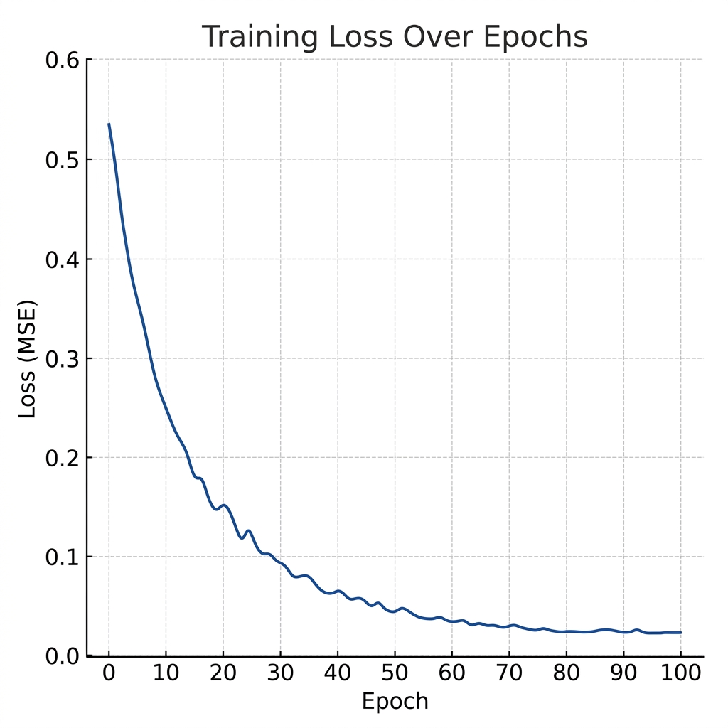
As training progresses, the loss steadily decreases. The network is literally "learning" — adjusting its internal weights so its predictions get closer and closer to the true labels.
5. A Worked Numerical Example
Let's trace through one complete forward + backward pass with concrete numbers for the XOR problem with input $(1, 0)$ and target $y = 1$.
Initial weights (randomly chosen):
- Hidden weights: $W_1 = \begin{bmatrix} 0.5 & -0.3 \\ 0.2 & 0.8 \\ -0.4 & 0.6 \end{bmatrix}$, biases: $b_h = [0.1, -0.1, 0.2]$
- Output weights: $W_2 = [0.7, -0.5, 0.3]$, bias: $b_o = 0.1$
Forward pass:
- $z_{h_1} = 0.5(1) + (-0.3)(0) + 0.1 = 0.6 \quad \Rightarrow \quad a_{h_1} = \sigma(0.6) = 0.6457$
- $z_{h_2} = 0.2(1) + 0.8(0) + (-0.1) = 0.1 \quad \Rightarrow \quad a_{h_2} = \sigma(0.1) = 0.5250$
- $z_{h_3} = -0.4(1) + 0.6(0) + 0.2 = -0.2 \quad \Rightarrow \quad a_{h_3} = \sigma(-0.2) = 0.4502$
- $z_o = 0.7(0.6457) + (-0.5)(0.5250) + 0.3(0.4502) + 0.1 = 0.3946$
- $\hat{y} = \sigma(0.3946) = 0.5974$
- $\mathcal{L} = \frac{1}{2}(1 - 0.5974)^2 = 0.0810$
Backward pass (for output weight $w_{o_1} = 0.7$):
- $\frac{\partial \mathcal{L}}{\partial \hat{y}} = -(1 - 0.5974) = -0.4026$
- $\frac{\partial \hat{y}}{\partial z_o} = 0.5974 \times 0.4026 = 0.2405$
- $\frac{\partial z_o}{\partial w_{o_1}} = a_{h_1} = 0.6457$
- $\frac{\partial \mathcal{L}}{\partial w_{o_1}} = (-0.4026)(0.2405)(0.6457) = -0.0625$
With learning rate $\alpha = 0.5$:
$$w_{o_1}^{\text{new}} = 0.7 - 0.5 \times (-0.0625) = 0.7313$$
The weight increased slightly, which will push the prediction closer to the target of 1 on the next forward pass.
6. Complete Python Implementation from Scratch
Here is a fully working neural network that learns XOR using nothing but NumPy:
import numpy as np

# ---- Activation & its derivative ----
def sigmoid(z):
    return 1 / (1 + np.exp(-z))

def sigmoid_deriv(a):
    """Derivative of sigmoid given its output 'a'."""
    return a * (1 - a)

# ---- XOR Dataset ----
X = np.array([[0, 0],
              [0, 1],
              [1, 0],
              [1, 1]])

y = np.array([[0], [1], [1], [0]])

# ---- Network Architecture ----
np.random.seed(42)
input_size  = 2
hidden_size = 4
output_size = 1
lr = 0.5           # Learning rate
epochs = 10000

# Initialize weights & biases randomly
W1 = np.random.randn(input_size, hidden_size) * 0.5
b1 = np.zeros((1, hidden_size))
W2 = np.random.randn(hidden_size, output_size) * 0.5
b2 = np.zeros((1, output_size))

# ---- Training Loop ----
losses = []
for epoch in range(epochs):

    # ==== FORWARD PROPAGATION ====
    # Hidden layer
    z1 = X @ W1 + b1           # (4, 4) weighted sum
    a1 = sigmoid(z1)            # (4, 4) activations

    # Output layer
    z2 = a1 @ W2 + b2           # (4, 1) weighted sum
    a2 = sigmoid(z2)            # (4, 1) prediction (y_hat)

    # Loss (MSE)
    loss = np.mean((y - a2) ** 2)
    losses.append(loss)

    # ==== BACKWARD PROPAGATION ====
    # Output layer gradients
    dL_da2 = -(y - a2)                           # (4, 1)
    da2_dz2 = sigmoid_deriv(a2)                   # (4, 1)
    delta2 = dL_da2 * da2_dz2                     # (4, 1)

    dL_dW2 = a1.T @ delta2                        # (4, 1)
    dL_db2 = np.sum(delta2, axis=0, keepdims=True) # (1, 1)

    # Hidden layer gradients (chain rule continues)
    dL_da1 = delta2 @ W2.T                        # (4, 4)
    da1_dz1 = sigmoid_deriv(a1)                    # (4, 4)
    delta1 = dL_da1 * da1_dz1                      # (4, 4)

    dL_dW1 = X.T @ delta1                          # (2, 4)
    dL_db1 = np.sum(delta1, axis=0, keepdims=True)  # (1, 4)

    # ==== WEIGHT UPDATE (Gradient Descent) ====
    W2 -= lr * dL_dW2
    b2 -= lr * dL_db2
    W1 -= lr * dL_dW1
    b1 -= lr * dL_db1

    if (epoch + 1) % 2000 == 0:
        print(f"Epoch {epoch+1:5d} | Loss: {loss:.6f}")

# ---- Final Predictions ----
print("\n--- Final Predictions ---")
for i in range(len(X)):
    print(f"Input: {X[i]}  |  Predicted: {a2[i][0]:.4f}  |  Target: {y[i][0]}")
Expected output after training:
Epoch  2000 | Loss: 0.032841
Epoch  4000 | Loss: 0.007132
Epoch  6000 | Loss: 0.003614
Epoch  8000 | Loss: 0.002329
Epoch 10000 | Loss: 0.001692

--- Final Predictions ---
Input: [0 0]  |  Predicted: 0.0380  |  Target: 0
Input: [0 1]  |  Predicted: 0.9612  |  Target: 1
Input: [1 0]  |  Predicted: 0.9610  |  Target: 1
Input: [1 1]  |  Predicted: 0.0434  |  Target: 0
The network has successfully learned the XOR function — a problem impossible for a single neuron — by learning the right weights through thousands of forward and backward passes.
7. Key Takeaways
- Forward propagation computes predictions by passing data through weighted sums and activation functions, layer by layer.
- Backward propagation uses the chain rule to compute exactly how much each weight contributed to the error.
- Gradient descent uses these gradients to nudge every weight in the direction that reduces the loss.
- The learning rate controls step size — it's one of the most critical hyperparameters to tune.
- Modern frameworks like PyTorch and TensorFlow handle backprop automatically via autograd, but understanding the math gives you the intuition to debug and design better architectures.